Characteristics of a Time Series Data

 3 key characteristics of a Time Series Data: 

Stationarity, Trend and Seasonality.

1. Stationarity:

Stationarity is on demand for almost every time series analysis use case because it is stable to analyze. Moreover, there are useful modeling techniques that require a time series to be stationary, such as Auto Regressive (AR) or Moving Average (MA). So, basically what is stationary and how do we know (or test) if a time series has this characteristic?

A strictly stationary time series is one for which the probabilistic behavior of every collection of values is identical to that of the time shifted set. [1]

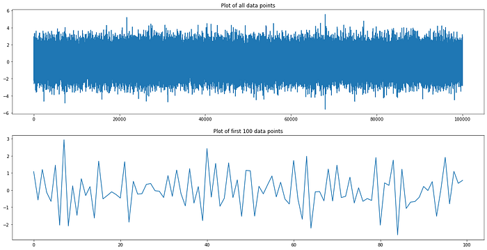
But for most cases, people refer to stationary characteristics with a less formal definition by saying the mean and the variance of a time series does not change over time. If you take a shifted sample from an original time series at any lag or lead, you would likely get the same distribution.

The former characteristic is known as strictly stationarity. However in practice, the definition is too strong for most applications. As a result, data scientists usually refer to a more looser version of stationarity, which is called weakly stationary:

A weakly stationary time series, x_t , is a finite variance process such that
(i) the mean value function, μ_t , defined in (1.9) is constant and does not depend on time t
(ii) the autocovariance function, γ(s, t), defined in (1.10) depends on s and t only through their difference |s − t|. [2]

The latter condition introduces a new concept — the autocovariance function. The term reminds us of covariance, which is a much more familiar measurement that determines how well 2 series vary together. The large absolute value of covariance denotes the strong relationships between these 2 in either positive or negative direction. With regard to autocovariance, it is simply the covariance of a time series and a lagged version of itself, which is used to evaluate the effect of the past observations on the later ones within a single time series. In fact, in many practical cases, the last values in the past might be useful at some point to forecast those in the future.

Figure 1. A stationary time series example

How do we test if a series is stationary? Several testing techniques can be conducted to check for the characteristics, such as Augmented Dickey Fuller (ADF) test or Kwiatkowski–Phillips–Schmidt–Shin (KPSS) test. Although ADF is more commonly used as a statistical tool to verify stationarity, what it actually tests is whether a time series contains a unit root or not. This may lead to a scenario where the test does not yield the expected result. However, I would not go into detail here.

2. Trend

For many cases in the world where the data shows an upward or downward trend over time, we might be interested in analyzing these patterns. For example, a company’s stock price has witnessed an incline for the past 30 years, or the decline in the birth rate of a country in the last decade.

Figure 2. An example of a trend time series (bottom) with the linear trend pattern (top)

Why is the trend important ?

In the long run, if the trend is predictable, it may allow us to capture the main direction of the time series data, hence leading to a better future forecast. Imagine while stationarity enables data scientists to include the day-by-day (period-by-period) effect of the series, it is the trend that helps to detect the long term movement.

When a series contains an implicit trend, the mean is observed to change over time. As you extract the data in different periods, you are likely to retrieve different mean values. Therefore, a trend time series is non-stationary regarding the definition.

There are several typical types of trends that we might encounter in practice. The most popular one is a linear trend where the data seem to fluctuate around a line. Besides, a quadratic trend, an exponential trend might sometimes occur for a time series where the increase in the time steps refers to a quicker and quicker growth or decline of the observed values.

What to do if we observe a trend in practice ?

For most of the time, data scientists make the effort to decompose the trend out of the original series to analyze it separately. Some transformation could be applied, such as regression or differencing, which results in a new series that is likely to be stationary (Sometimes it does require more transformation and seasonality removal).

3. Seasonality

While the stationary characteristic aims at analyzing day-by-day (period-by-period) relationships, seasonality captures the regular pattern within an interval (usually less than a year). For instance, the sale of swimsuits in Vietnam shows a peak in every summer and a valley in every winter, and this behavior is repeated in many years. Note that the preceding example shows the variance between actual yearly seasons, however, the term “seasonality” could be understood to a smaller or larger fix period, such as a week, a month, a half of a year, as long as it stays within a year.

Figure 3. An example of a seasonal time series (bottom) with the decomposed seasonal pattern (top)

Seasonality makes the time series data vary across seasons, which is a sign of time-dependence. Consequently, a seasonal time series is non-stationary. As we decompose the trend to make a series stationary, we would do the same with seasonality. The most popular technique is to difference the sequence by period of the seasonal interval. For example, the swimsuit sale data has the seasonal period equal to 1 year. If the series is daily sampled, we could difference it with a 365-day shifted one. The transformation would result in a time series data with seasonality characteristics removed.

Content adopted from medium.com.